
| 일 | 월 | 화 | 수 | 목 | 금 | 토 |
|---|---|---|---|---|---|---|
| 1 | ||||||
| 2 | 3 | 4 | 5 | 6 | 7 | 8 |
| 9 | 10 | 11 | 12 | 13 | 14 | 15 |
| 16 | 17 | 18 | 19 | 20 | 21 | 22 |
| 23 | 24 | 25 | 26 | 27 | 28 | 29 |
| 30 |
- tensorflow
- 코딩테스트
- 선형회귀
- 회귀
- PyTorch
- Linear
- 재귀함수
- 템플릿
- 연습
- 기초
- 흐름도
- 딥러닝
- 추천시스템
- 게임
- 머신러닝
- 가격맞히기
- 프로그래머스
- Regression
- 코딩
- 파이썬
- CLI
- 주식연습
- 크롤링
- python
- API
- 주가예측
- DeepLearning
- 알고리즘
- 주식매매
- 주식
- Today
- Total
코딩걸음마
[딥러닝] TensorFlow+ 분류모델 예제(MNIST) 본문

이번엔 회귀모델이 아니라 텐서플로우를 활용하여 딥러닝 분류를 알아봅시다.
다음의 이미지를 봅시다.
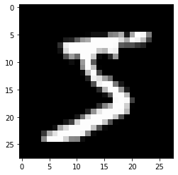
사람은 이 그림이 5라는 것을 당연하게 빠르게 답변할 수 있습니다.
하지만 컴퓨터는 알아내지 못한다. 그렇다면 컴퓨터는 어떻게 보일까요?
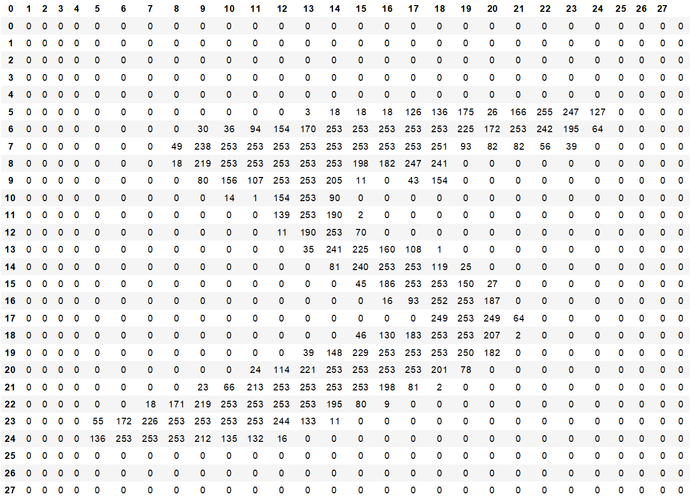
컴퓨터는 하얀부분을 255 검은부분을 0이라는 규칙을 가지고 0~255사이의 값을 가진 Data로 표현됩니다.
즉 , 하나의 그림 안은 28개 열과, 28개 행의 Data 즉, 784개의 Data의 vector(지금은 Matrix)라고 표현할 수 있습니다.
1. 데이터 준비
우선 data를 불러옵시다.
import tensorflow as tf
from tensorflow.keras import datasets, models, layers, utils, losses
import os
os.environ['TF_CPP_MIN_LOG_LEVEL'] = '2' # https://stackoverflow.com/questions/35911252/disable-tensorflow-debugging-information
(train_data, train_label), (test_data, test_label) = datasets.mnist.load_data()Data의 크기를 알아봅시다.
print(train_data.shape)
print(test_data.shape)
(60000, 28, 28)
(10000, 28, 28)1개의 그림에는 784개의 Data가 있고 (28*28) 그 그림이 70,000개가 있습니다.
그중 10,000개는 test_data로 분리하여 사용할 것입니다.
분석을 위해 차원을 변경해봅시다.
정확도를 높히기 위해 data 값을 scaling 해야합니다.
명암의 값은 0~255범위의 값을 가지므로 255로 나누어 값을 일반화 시킵니다.
train_data = train_data.reshape(60000, 28*28) / 255.0
test_data = test_data.reshape(10000, 28*28) / 255.0
(28,28) 크기의 Matrix였던 그림을 784개의 data를 가진 vector로 변환합니다.
train_data.shape(60000, 784)
다음은 label data를 전처리할 단계입니다.
train_labelarray([5, 0, 4, ..., 5, 6, 8], dtype=uint8)현재 label 은 int 형식이며 각 행에 1개의 data를 가지고 있습니다.
분류를 위해 각 label을 integer value에서 one-hot vector로 변경해줍니다.
OHS해봅시다.
train_label = utils.to_categorical(train_label) # 0~9 -> one-hot vector
test_label = utils.to_categorical(test_label) # 0~9 -> one-hot vector
train_labelarray([[0., 0., 0., ..., 0., 0., 0.],
[1., 0., 0., ..., 0., 0., 0.],
[0., 0., 0., ..., 0., 0., 0.],
...,
[0., 0., 0., ..., 0., 0., 0.],
[0., 0., 0., ..., 0., 0., 0.],
[0., 0., 0., ..., 0., 1., 0.]], dtype=float32)2. 모델 설정
from keras.models import Sequential
from keras.layers import Dense, Activation
model = models.Sequential() # "Sequence" (Linear stack of layers)Sequential() 클래스를 상속받은 model 객체를 생성합니다.
Sequential()은 연속적으로 선형결합층을 쌓을 수 있는 바탕이라고 생각하시면됩니다.
model.add(layers.Dense(input_dim=28*28, units=512, activation='relu', kernel_initializer='he_uniform')) # Dense-layer (relu & he)
model.add(layers.Dropout(0.2)) # Dropout-layer
model.add(layers.Dense(units=10, activation='softmax')) # (Output) Dense-layer with softmax function, 0~9 -> 10
위 코드를 자세히 알아봅시다.
model.add(layers.Dense(input_dim=28*28, units=512, activation='relu', kernel_initializer='he_uniform'))
input_dim = 입력 값 개수
units = 출력 값 개수
activation = 입력된 값들을 비선형 함수에 통과시킨 후 다음 레이어로 전달하는데, 이 때 사용하는 함수
kernel_initializer= 초기 난수 가중치를 설정하는 방식을 뜻합니다..
model.add(layers.Dropout(0.2))
모델에 Dropout 함수를 적용할 경우, 과적합을 방지하기 위해 무작위로 특정 노드(입력값)를 0으로 만듭니다.
무작위 노드를 비활성화 시킵니다. 마치 타노스 처럼요

model.add(layers.Dense(units=10, activation='softmax'))
softmax = 소프트맥스 함수는 로지스틱 함수의 다차원 일반화입니다. 다항 로지스틱 회귀에서 쓰이고, 인공신경망에서 확률분포를 얻기 위한 마지막 활성함수로 많이 사용됩니다.
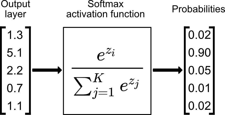
결과 값은 0~9범위로 10개가 있으므로 units=10으로 설정합니다.
모델 확인하기
model.summary()Model: "sequential_2"
_________________________________________________________________
Layer (type) Output Shape Param #
=================================================================
dense_4 (Dense) (None, 512) 401920
_________________________________________________________________
dropout_2 (Dropout) (None, 512) 0
_________________________________________________________________
dense_5 (Dense) (None, 10) 5130
=================================================================
Total params: 407,050
Trainable params: 407,050
Non-trainable params: 0
______________________________________참고) 다음은 모델 유형별 출력노드와 실행함수들입니다.
# Regression
model.add(layers.Dense(units=1, activation=None))
model.compile(optimizer='adam',
              loss=losses.mean_squared_error,
              metrics=['mean_squared_error'])

# Multi-class classification
model.add(layers.Dense(units=10, activation='softmax'))
model.compile(optimizer='adam',
              loss=losses.categorical_crossentropy,        # <- Label이 One-hot 형태일 경우
              loss=losses.sparse_categorical_crossentropy, # <- Label이 One-hot 형태가 아닐 경우
              metrics=['accuracy'])

# Binary Classification 1 (Softmax를 적용하는 경우, recommended)
model.add(layers.Dense(units=2, activation='softmax'))
model.compile(optimizer='adam',
              loss=losses.categorical_crossentropy,
              metrics=['accuracy'])

# Binary Classification 2 (Sigmoid를 적용하는 경우)
# 선형결합 결과에 대해 sigmoid function의 output을 계산해주면, binary_crossentropy가 이를 음성 & 양성 확률로 변환하여 처리해줍니다.
model.add(layers.Dense(units=1, activation='sigmoid'))
model.compile(optimizer='adam',
              loss=losses.binary_crossentropy,
              metrics=['accuracy'])
3. 모델 실행
이제 모델을 실행해봅시다.
model.compile 로 실행하는데 다음의 세부사항을 설정해주어야합니다.
# "Compile" the model description (Configures the model for training)
model.compile(optimizer='adam',
              loss=losses.categorical_crossentropy, # See other available losses @ https://keras.io/losses/
              metrics=['accuracy']) # TF 2.X 에서 Precision / Recall / F1-Score 적용하기 @ https://j.mp/3cf3lbi
optimizer = 학습 데이터(Train data)셋을 이용하여 모델을 학습 할 때 데이터의 실제 결과와 모델이 예측한 결과를 기반으로 잘 줄일 수 있게 만들어주는 역할을 합니다.
loss = 목표가 되는 함수 입니다. 여기서는 교차엔트로피함수를 사용해서 loss를 줄이고자 합니다.
4. 모델 훈련
# Fit the model on training data

model.fit(train_data, train_label, batch_size=100, epochs=10) # default batch_size = 32
#model.fit(train_data, train_label, batch_size=100, epochs=15, validation_split=0.2)
Epoch 1/10
600/600 [==============================] - 2s 3ms/step - loss: 0.2644 - accuracy: 0.9244
Epoch 2/10
600/600 [==============================] - 2s 3ms/step - loss: 0.1130 - accuracy: 0.9662
........
Epoch 9/10
600/600 [==============================] - 2s 3ms/step - loss: 0.0227 - accuracy: 0.9926
Epoch 10/10
600/600 [==============================] - 2s 3ms/step - loss: 0.0197 - accuracy: 0.9934
5. 모델 평가
# Evaluate the model on test data

result = model.evaluate(test_data, test_label, batch_size=100)
100/100 [==============================] - 0s 2ms/step - loss: 0.0602 - accuracy: 0.9830
print('loss (cross-entropy) :', result[0])
print('test accuracy :', result[1])
loss (cross-entropy) : 0.06631594151258469
test accuracy : 0.9801999926567078
6. 모델 사용
model.predict(test_data[0:1,:])array([[5.1109810e-09, 9.2115995e-11, 1.4228991e-07, 1.3642444e-04,
2.7073114e-13, 2.2115463e-08, 8.8259472e-13, 9.9986136e-01,
1.1195265e-08, 2.0405787e-06]], dtype=float32)
7. 모델 템플릿
위 코드 요약
# 1. Normalization
(train_data, train_label), (test_data, test_label) = datasets.mnist.load_data()

# 각 이미지를 [28행 x 28열]에서 [1행 x 784열]로 펼쳐줍니다.
# 각 이미지 내의 pixel 값을 [0~255]에서 [0~1]로 바꿔줍니다.

train_data = train_data.reshape(60000, 28*28) / 255.0
test_data = test_data.reshape(10000, 28*28) / 255.0

# 각 label을 integer value에서 one-hot vector로 변경해줍니다. (Tensorflow 2.x 활용)
train_label = utils.to_categorical(train_label) # 0~9 -> one-hot vector
test_label = utils.to_categorical(test_label) # 0~9 -> one-hot vector

# 2. Build the model & Set the criterion
model = models.Sequential() # Build up the "Sequence" of layers (Linear stack of layers)
model.add(layers.Dense(input_dim=28*28, units=512, activation='relu', kernel_initializer='he_uniform')) # Dense-layer (relu & he)
model.add(layers.Dropout(0.2)) # Dropout-layer
model.add(layers.Dense(units=10, activation='softmax')) # (Output) Dense-layer with softmax function, 0~9 -> 10

# 3. "Compile" the model description (Configures the model for training)
model.compile(optimizer='adam',
              loss=losses.categorical_crossentropy, # See other available losses @ https://keras.io/losses/
              metrics=['accuracy']) # TF 2.X 에서 Precision / Recall / F1-Score 적용하기 @ https://j.mp/3cf3lbi

print(model.summary())

# 4. Train the model
# Fit the model on training data
model.fit(train_data, train_label, batch_size=100, epochs=10) # default batch_size = 32

# 5.  Test the model
# Evaluate the model on test data
result = model.evaluate(test_data, test_label, batch_size=100)
print('loss (cross-entropy) :', result[0])
print('test accuracy :', result[1])
tf.keras.layers.Flatten() 활용
입력을 1차원으로 변환합니다.Batch의 크기에는 영향을 주지 않습니다.
(train_data, train_label), (test_data, test_label) = datasets.mnist.load_data()

# 아래 코드에서 reshape 적용을 생략하고, 대신 Flatten 레이어를 활용해 펼쳐낼 수 있습니다.
# train_data = train_data.reshape(60000, 784) / 255.0
# test_data = test_data.reshape(10000, 784) / 255.0

train_data = train_data / 255.0
test_data = test_data / 255.0

train_label = utils.to_categorical(train_label)
test_label = utils.to_categorical(test_label)


model = models.Sequential()

model.add(layers.Flatten()) # takes our 28x28 and makes it 1x784

# model.add(layers.Dense(input_dim=28*28, units=512, activation='relu', kernel_initializer='he_uniform'))
model.add(layers.Dense(units=512, activation=tf.nn.relu, kernel_initializer='he_uniform')) # tf.nn 활용이 가능합니다.
model.add(layers.Dropout(0.2))
model.add(layers.Dense(units=10, activation=tf.nn.softmax)) # tf.nn 활용이 가능합니다.

model.compile(optimizer='adam',
              loss=losses.categorical_crossentropy,
              metrics=['accuracy'])

model.fit(train_data, train_label, batch_size=100, epochs=10)

result = model.evaluate(test_data, test_label, batch_size=100)
print('loss (cross-entropy) :', result[0])
print('test accuracy :', result[1])
+BatchNormalization +validation + 시각화
BatchNormalization = 학습하는 과정 자체를 전체적으로 안정화하여 학습 속도를 가속 시킬 수 있는 근본적인 방법
import tensorflow as tf
from tensorflow.keras import datasets, utils
from tensorflow.keras import models, layers, activations, initializers, losses, optimizers, metrics

import os
os.environ['TF_CPP_MIN_LOG_LEVEL'] = '2'


# 1. Normalization
(train_data, train_label), (test_data, test_label) = datasets.mnist.load_data()

# 각 이미지를 [28행 x 28열]에서 [1행 x 784열]로 펼쳐줍니다.
# 각 이미지 내의 pixel 값을 [0~255]에서 [0~1]로 바꿔줍니다.

train_data = train_data.reshape(60000, 28*28) / 255.0
test_data = test_data.reshape(10000, 28*28) / 255.0

# 각 label을 integer value에서 one-hot vector로 변경해줍니다. (Tensorflow 2.x 활용)
train_label = utils.to_categorical(train_label) # 0~9 -> one-hot vector
test_label = utils.to_categorical(test_label) # 0~9 -> one-hot vector

# 2. Build the model & Set the criterion + Batch_Normalization
model = models.Sequential()

model.add(layers.Dense(input_dim=28*28, units=256, activation=None, kernel_initializer=initializers.he_uniform()))
model.add(layers.BatchNormalization())
model.add(layers.Activation('relu')) # layers.ELU or layers.LeakyReLU
model.add(layers.Dropout(rate=0.2))

model.add(layers.Dense(units=256, activation=None, kernel_initializer=initializers.he_uniform()))
model.add(layers.BatchNormalization())
model.add(layers.Activation('relu')) # layers.ELU or layers.LeakyReLU
model.add(layers.Dropout(rate=0.2))

model.add(layers.Dense(units=10, activation='softmax')) # 0~9

# 3. "Compile" the model description (Configures the model for training)
model.compile(optimizer=optimizers.Adam(),
              loss=losses.categorical_crossentropy,
              metrics=[metrics.categorical_accuracy]) # Precision / Recall / F1-Score 적용하기 @ https://j.mp/3cf3lbi

# model.compile(optimizer='adam',
#               loss=losses.categorical_crossentropy,
#               metrics=['accuracy'])
print(model.summary())

# 4. Train the model
# Fit the model on training data
# Training 과정에서 epoch마다 활용할 validation set을 나눠줄 수 있습니다.
history = model.fit(train_data, train_label, batch_size=100, epochs=15, validation_split=0.2)

# 5.  Test the model
# Evaluate the model on test data
result = model.evaluate(test_data, test_label, batch_size=100)

print('loss (cross-entropy) :', result[0])
print('test accuracy :', result[1])

# 6. Visualize the result
val_acc = history.history['val_categorical_accuracy']
acc = history.history['categorical_accuracy']

import numpy as np
import matplotlib.pyplot as plt

x_len = np.arange(len(acc))
plt.plot(x_len, acc, marker='.', c='blue', label="Train-set Acc.")
plt.plot(x_len, val_acc, marker='.', c='red', label="Validation-set Acc.")

plt.legend(loc='upper right')
plt.grid()
plt.xlabel('epoch')
plt.ylabel('Accuracy')
plt.show()
값을 활용하여 추정하기
model.predict(test_data[0:1,:])array([[1.1306721e-11, 1.4323449e-13, 3.0133476e-12, 8.9055938e-08,
1.7670583e-16, 5.2259764e-13, 8.2227857e-18, 9.9999988e-01,
1.7712066e-11, 8.4726492e-10]], dtype=float32)'딥러닝_TensorFlow' 카테고리의 다른 글
| [딥러닝] TensorFlow 모델 save / Load (+Keras Callback ) (0) | 2022.07.01 |
|---|---|
| [딥러닝] TensorFlow1.0 기초 + 회귀모델 예제 (0) | 2022.06.28 |

