
250x250
Notice
Recent Posts
Recent Comments
Link
| 일 | 월 | 화 | 수 | 목 | 금 | 토 |
|---|---|---|---|---|---|---|
| 1 | 2 | 3 | 4 | 5 | 6 | |
| 7 | 8 | 9 | 10 | 11 | 12 | 13 |
| 14 | 15 | 16 | 17 | 18 | 19 | 20 |
| 21 | 22 | 23 | 24 | 25 | 26 | 27 |
| 28 | 29 | 30 | 31 |
Tags
- 회귀
- 기초
- 주식연습
- 템플릿
- 주식매매
- Linear
- 머신러닝
- 파이썬
- 코딩테스트
- 크롤링
- 게임
- 재귀함수
- PyTorch
- CLI
- 알고리즘
- 흐름도
- DeepLearning
- 프로그래머스
- 추천시스템
- 선형회귀
- 가격맞히기
- API
- 주식
- 딥러닝
- 주가예측
- python
- 코딩
- Regression
- 연습
- tensorflow
Archives
- Today
- Total
코딩걸음마
[딥러닝-예제] 선형회귀 (Linear Regression) (보스턴 주택가격예측) 본문
728x90
1. Data 불러오기
!pip install matplotlib seaborn pandas sklearn
import pandas as pd
import seaborn as sns
import matplotlib.pyplot as plt
선형회귀에 사용할 sample은 유명한 boston 주택가격 예측입니다.
from sklearn.datasets import load_boston
boston = load_boston()

print(boston.DESCR)
2. Data 확인하기
.. _boston_dataset:

Boston house prices dataset
---------------------------

**Data Set Characteristics:**

    :Number of Instances: 506

    :Number of Attributes: 13 numeric/categorical predictive. Median Value (attribute 14) is usually the target.

    :Attribute Information (in order):
        - CRIM     per capita crime rate by town
        - ZN       proportion of residential land zoned for lots over 25,000 sq.ft.
        - INDUS    proportion of non-retail business acres per town
        - CHAS     Charles River dummy variable (= 1 if tract bounds river; 0 otherwise)
        - NOX      nitric oxides concentration (parts per 10 million)
        - RM       average number of rooms per dwelling
        - AGE      proportion of owner-occupied units built prior to 1940
        - DIS      weighted distances to five Boston employment centres
        - RAD      index of accessibility to radial highways
        - TAX      full-value property-tax rate per $10,000
        - PTRATIO  pupil-teacher ratio by town
        - B        1000(Bk - 0.63)^2 where Bk is the proportion of blacks by town
        - LSTAT    % lower status of the population
        - MEDV     Median value of owner-occupied homes in $1000's

    :Missing Attribute Values: None

    :Creator: Harrison, D. and Rubinfeld, D.L.

This is a copy of UCI ML housing dataset.
https://archive.ics.uci.edu/ml/machine-learning-databases/housing/


This dataset was taken from the StatLib library which is maintained at Carnegie Mellon University.

The Boston house-price data of Harrison, D. and Rubinfeld, D.L. 'Hedonic
prices and the demand for clean air', J. Environ. Economics & Management,
vol.5, 81-102, 1978.   Used in Belsley, Kuh & Welsch, 'Regression diagnostics
...', Wiley, 1980.   N.B. Various transformations are used in the table on
pages 244-261 of the latter.

The Boston house-price data has been used in many machine learning papers that address regression
problems.

.. topic:: References

   - Belsley, Kuh & Welsch, 'Regression diagnostics: Identifying Influential Data and Sources of Collinearity', Wiley, 1980. 244-261.
   - Quinlan,R. (1993). Combining Instance-Based and Model-Based Learning. In Proceedings on the Tenth International Conference of Machine Learning, 236-243, University of Massachusetts, Amherst. Morgan Kaufmann.
df를 불러옵니다.
df = pd.DataFrame(boston.data, columns=boston.feature_names)df.columnsIndex(['CRIM', 'ZN', 'INDUS', 'CHAS', 'NOX', 'RM', 'AGE', 'DIS', 'RAD', 'TAX',
'PTRATIO', 'B', 'LSTAT'],
dtype='object')df.info()<class 'pandas.core.frame.DataFrame'>
RangeIndex: 506 entries, 0 to 505
Data columns (total 13 columns):
# Column Non-Null Count Dtype
--- ------ -------------- -----
0 CRIM 506 non-null float64
1 ZN 506 non-null float64
2 INDUS 506 non-null float64
3 CHAS 506 non-null float64
4 NOX 506 non-null float64
5 RM 506 non-null float64
6 AGE 506 non-null float64
7 DIS 506 non-null float64
8 RAD 506 non-null float64
9 TAX 506 non-null float64
10 PTRATIO 506 non-null float64
11 B 506 non-null float64
12 LSTAT 506 non-null float64
dtypes: float64(13)
memory usage: 51.5 KB결측치가 하나도 없이 깔끔하고 Dtype이 모두 float64로 분석하기에 좋습니다.
df = pd.DataFrame(boston.data, columns=boston.feature_names)
df["target"] = boston.target
df.tail()
df["target"] 컬럼을 생성합시다. boston.target이 바로 목표로 하는 컬럼입니다.
시각화로 확인하기
sns.pairplot(df)
plt.show()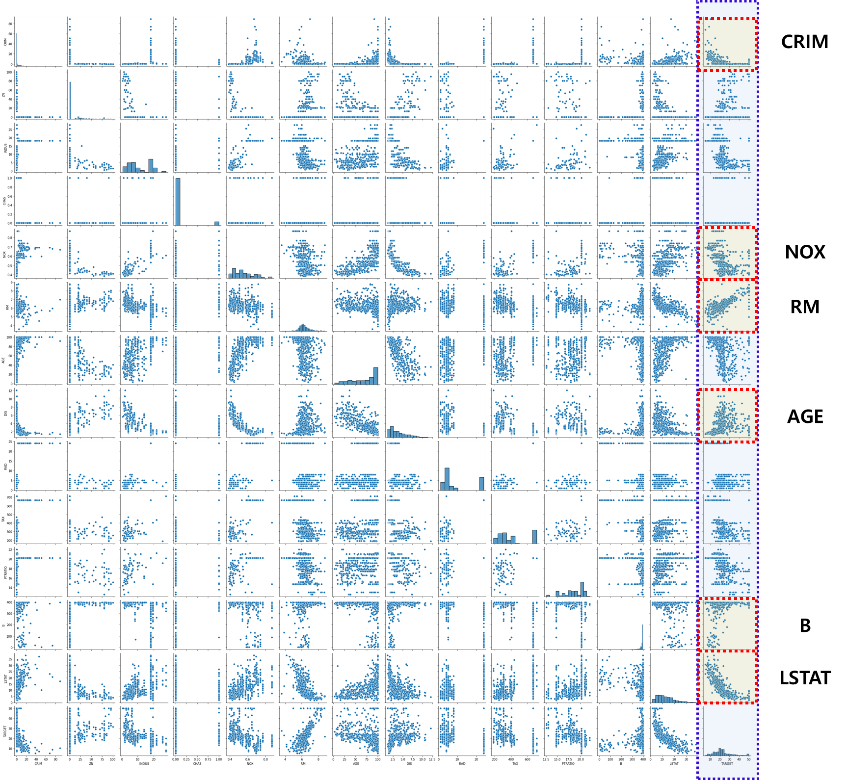
pairplot을 사용하여 target 컬럼과 선형관계가 보이는 컬럼을 따로 분리하여 딥러닝을 작동시켜보자
cols = ["TARGET", "CRIM", "NOX", "RM", "AGE", "B", "LSTAT"]
3. Train Linear Model with PyTorch
import torch
import torch.nn as nn
import torch.nn.functional as F
import torch.optim as optim
data = torch.from_numpy(df[cols].values).float()

data.shape
torch.Size([506, 7])df[cols].values : df 내 모든 컬럼의 값을 출력합니다.
위 코드로 출력하면, np.array 형태로 나오기 때문에 torch.from_numpy로 tensor로 무조건 변경해줘야 합니다.
target data와 train data로 분리합니다.
# Split x and y.
y = data[:, :1]
x = data[:, 1:]

print(x.shape, y.shape)
torch.Size([506, 5]) torch.Size([506, 1])
4. Model Define
# Define configurations.
n_epochs = 20000
learning_rate = 1e-4
print_interval = 500
n_epochs 몇 번을 반복 학습할 것인지 정하는 hyper params입니다.
learning_rate는 한번의 학습으로 함수 내 parameter들을 얼마나 변경시킬 것인지 정하는 hyper params입니다.
data를 모델에 적용합니다. (≒ 머신러닝의 model.fit() )
nn.Linear 클래스의 객체로서 model을 선언해줍니다.
# Define model.
model = nn.Linear(x.size(-1), y.size(-1))

model
Linear(in_features=5, out_features=1, bias=True)
다음은 최적화함수를 설정해줍니다. sigmoid 함수를 활용하여 최적화 해주도록 합시다.
# Instead of implement gradient equation,
# we can use <optim class> to update model parameters, automatically.
optimizer = optim.SGD(model.parameters(),
                      lr=learning_rate)
모델 가동
# Whole training samples are used in 1 epoch.
# Thus, "N epochs" means that model saw a sample N-times.
loss_list = [ ]
Epoch_list = [ ]
for i in range(n_epochs):
    y_hat = model(x)
    loss = F.mse_loss(y_hat, y)

    optimizer.zero_grad()
    loss.backward()

    optimizer.step()

    if (i + 1) % print_interval == 0:
        print('Epoch %d: loss=%.4e' % (i + 1, loss))
        loss_list.append(loss)
        Epoch_list.append(i+1)
Epoch 500: loss=5.3882e+01
Epoch 1000: loss=4.4285e+01
Epoch 1500: loss=4.0388e+01
Epoch 2000: loss=3.7552e+01
Epoch 2500: loss=3.5425e+01
........
Epoch 18000: loss=2.9002e+01
Epoch 18500: loss=2.9002e+01
Epoch 19000: loss=2.9001e+01
Epoch 19500: loss=2.9001e+01
Epoch 20000: loss=2.9000e+01plt.plot(Epoch_list,loss_list)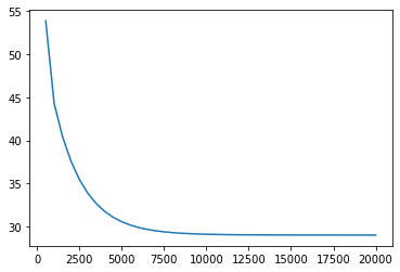
5. Model result
losstensor(29.0003, grad_fn=<MseLossBackward0>)
df = pd.DataFrame(torch.cat([y, y_hat], dim=1).detach_().numpy(),
                  columns=["y", "y_hat"])

sns.pairplot(df, height=5)
plt.show()
728x90
'딥러닝_Pytorch' 카테고리의 다른 글
| [딥러닝-예제] 선형회귀 (Linear Regression) (당뇨병 예측) (0) | 2022.06.27 |
|---|---|
| [딥러닝] Mean Square Error (MSE) Loss (0) | 2022.06.27 |
| [딥러닝] Pytorch 선형결합층(Linear_layer) (0) | 2022.06.26 |
| [딥러닝] Pytorch 행렬/텐서의 곱셈(Matrix/tensor Multiplication) (0) | 2022.06.24 |
| [딥러닝] Pytorch 주요함수 expand/randperm/argmax/topk/masked_fill/Ones , Zeros (0) | 2022.06.24 |
'딥러닝_Pytorch' Related Articles
more


Comments