
250x250
Notice
Recent Posts
Recent Comments
Link
| 일 | 월 | 화 | 수 | 목 | 금 | 토 |
|---|---|---|---|---|---|---|
| 1 | 2 | 3 | 4 | |||
| 5 | 6 | 7 | 8 | 9 | 10 | 11 |
| 12 | 13 | 14 | 15 | 16 | 17 | 18 |
| 19 | 20 | 21 | 22 | 23 | 24 | 25 |
| 26 | 27 | 28 | 29 | 30 | 31 |
Tags
- DeepLearning
- 주식
- tensorflow
- 알고리즘
- 주식매매
- Linear
- 가격맞히기
- 기초
- 게임
- Regression
- CLI
- 코딩테스트
- 연습
- 크롤링
- 주가예측
- 회귀
- 재귀함수
- 파이썬
- 딥러닝
- 템플릿
- 코딩
- PyTorch
- python
- API
- 머신러닝
- 추천시스템
- 선형회귀
- 흐름도
- 프로그래머스
- 주식연습
Archives
- Today
- Total
코딩걸음마
[딥러닝-예제] 선형회귀 (Linear Regression) (당뇨병 예측) 본문
728x90
1. Data 불러오기
!pip install matplotlib seaborn pandas sklearn
import pandas as pd
import seaborn as sns
import matplotlib.pyplot as plt
선형회귀에 사용할 sample은 유명한 당뇨병 예측입니다.
원래는 분류식으로 활용을 해야 정확하지만, 회귀식으로 dataset을 사용해보겠습니다.
from sklearn.datasets import load_diabetes
diabetes = load_diabetes()

print(diabetes.DESCR)
2. Data 확인하기
.. _diabetes_dataset:

Diabetes dataset
----------------

Ten baseline variables, age, sex, body mass index, average blood
pressure, and six blood serum measurements were obtained for each of n =
442 diabetes patients, as well as the response of interest, a
quantitative measure of disease progression one year after baseline.

**Data Set Characteristics:**

  :Number of Instances: 442

  :Number of Attributes: First 10 columns are numeric predictive values

  :Target: Column 11 is a quantitative measure of disease progression one year after baseline

  :Attribute Information:
      - age     age in years
      - sex
      - bmi     body mass index
      - bp      average blood pressure
      - s1      tc, T-Cells (a type of white blood cells)
      - s2      ldl, low-density lipoproteins
      - s3      hdl, high-density lipoproteins
      - s4      tch, thyroid stimulating hormone
      - s5      ltg, lamotrigine
      - s6      glu, blood sugar level

Note: Each of these 10 feature variables have been mean centered and scaled by the standard deviation times `n_samples` (i.e. the sum of squares of each column totals 1).

Source URL:
https://www4.stat.ncsu.edu/~boos/var.select/diabetes.html

For more information see:
Bradley Efron, Trevor Hastie, Iain Johnstone and Robert Tibshirani (2004) "Least Angle Regression," Annals of Statistics (with discussion), 407-499.
(https://web.stanford.edu/~hastie/Papers/LARS/LeastAngle_2002.pdf)
df를 불러옵니다.
df = pd.DataFrame(diabetes.data, columns=diabetes.feature_names)df.columnsIndex(['age', 'sex', 'bmi', 'bp', 's1', 's2', 's3', 's4', 's5', 's6'], dtype='object')df.info()<class 'pandas.core.frame.DataFrame'>
RangeIndex: 442 entries, 0 to 441
Data columns (total 10 columns):
# Column Non-Null Count Dtype
--- ------ -------------- -----
0 age 442 non-null float64
1 sex 442 non-null float64
2 bmi 442 non-null float64
3 bp 442 non-null float64
4 s1 442 non-null float64
5 s2 442 non-null float64
6 s3 442 non-null float64
7 s4 442 non-null float64
8 s5 442 non-null float64
9 s6 442 non-null float64
dtypes: float64(10)
memory usage: 34.7 KB결측치가 하나도 없이 깔끔하고 Dtype이 모두 float64로 분석하기에 좋습니다.
df = pd.DataFrame(diabetes.data, columns=diabetes.feature_names)
df["target"] = diabetes.target
df.tail()
df["target"] 컬럼을 생성합시다. diabetes.target이 바로 목표로 하는 컬럼입니다.
시각화로 한번 확인해봅시다.
sns.pairplot(df)
plt.show()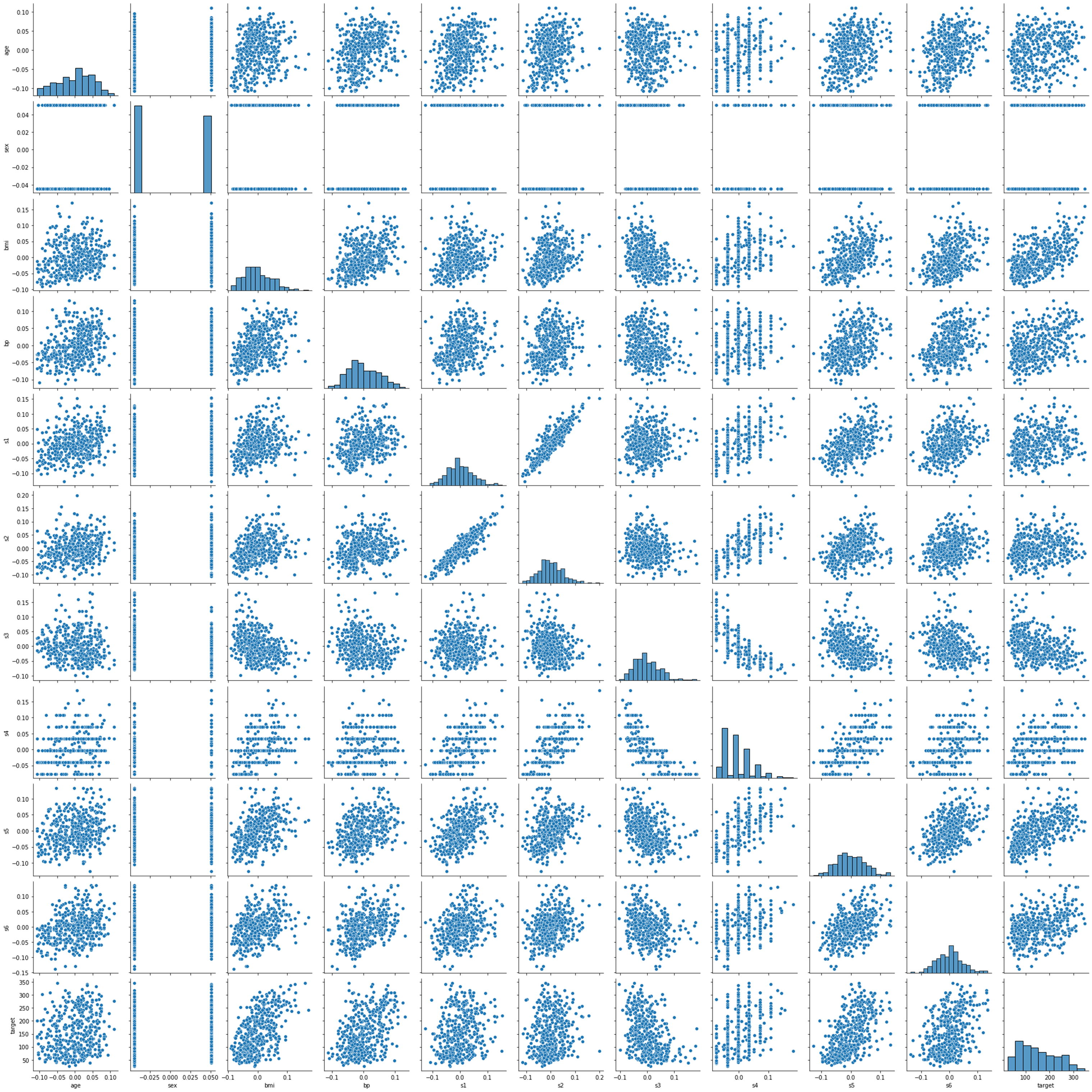
pairplot을 사용하여 보니 target과 선형성 보이지 않는 'sex','s4' 컬럼을 제거하고 분석해봅시다.
Index(['age', 'sex', 'bmi', 'bp', 's1', 's2', 's3', 's4', 's5', 's6',
       'target'],
      dtype='object')
cols = ['target','age', 'bmi', 'bp', 's1', 's2', 's3', 's5', 's6']
3. Train Linear Model with PyTorch
import torch
import torch.nn as nn
import torch.nn.functional as F
import torch.optim as optim
data = torch.from_numpy(df[cols].values).float()
data.shapetorch.Size([442, 9])df[cols].values : df 내 모든 컬럼의 값을 출력합니다.
위 코드로 출력하면, np.array 형태로 나오기 때문에 torch.from_numpy로 tensor로 무조건 변경해줘야 합니다.
target data와 train data로 분리합니다.
# Split x and y.
y = data[:, :1]
x = data[:, 1:]

print(x.shape, y.shape)
torch.Size([442, 8]) torch.Size([442, 1])
4. Model Define
# Define configurations.
n_epochs = 50000
learning_rate = 1e-3
print_interval = 500
n_epochs 몇 번을 반복 학습할 것인지 정하는 hyper params입니다.
learning_rate는 한번의 학습으로 함수 내 parameter들을 얼마나 변경시킬 것인지 정하는 hyper params입니다.
data를 모델에 적용합니다. (≒ 머신러닝의 model.fit() )
nn.Linear 클래스의 객체로서 model을 선언해줍니다.
# Define model.
model = nn.Linear(x.size(-1), y.size(-1))

model
Linear(in_features=8, out_features=1, bias=True)
다음은 최적화함수를 설정해줍니다. sigmoid 함수를 활용하여 최적화 해주도록 합시다.
# Instead of implement gradient equation,
# we can use <optim class> to update model parameters, automatically.
optimizer = optim.SGD(model.parameters(),
                      lr=learning_rate)
모델 가동
# Whole training samples are used in 1 epoch.
# Thus, "N epochs" means that model saw a sample N-times.
loss_list = [ ]
Epoch_list = [ ]
for i in range(n_epochs):
    y_hat = model(x)
    loss = F.mse_loss(y_hat, y)

    optimizer.zero_grad()
    loss.backward()

    optimizer.step()

    if (i + 1) % print_interval == 0:
        print('Epoch %d: loss=%.4e' % (i + 1, loss))
        loss_list.append(loss)
        Epoch_list.append(i+1)
Epoch 500: loss=9.0250e+03
Epoch 1000: loss=6.2836e+03
Epoch 1500: loss=5.8849e+03
Epoch 2000: loss=5.8029e+03
Epoch 2500: loss=5.7641e+03
Epoch 3000: loss=5.7316e+03
Epoch 3500: loss=5.7002e+03
....
Epoch 46000: loss=4.1018e+03
Epoch 46500: loss=4.0913e+03
Epoch 47000: loss=4.0810e+03
Epoch 47500: loss=4.0708e+03
Epoch 48000: loss=4.0607e+03
Epoch 48500: loss=4.0508e+03
Epoch 49000: loss=4.0409e+03
Epoch 49500: loss=4.0312e+03
Epoch 50000: loss=4.0216e+03plt.plot(Epoch_list,loss_list)
5. Model result
df = pd.DataFrame(torch.cat([y, y_hat], dim=1).detach_().numpy(),
                  columns=["y", "y_hat"])

sns.pairplot(df, height=5)
plt.show()
728x90
'딥러닝_Pytorch' 카테고리의 다른 글
| [딥러닝-예제] 선형회귀 (Linear Regression+deep neural network) (보스턴 주택가격예측) (0) | 2022.06.29 |
|---|---|
| [딥러닝-예제] 로지스틱 회귀 ( Logistic Regression) (유방암 예측) (0) | 2022.06.28 |
| [딥러닝] Mean Square Error (MSE) Loss (0) | 2022.06.27 |
| [딥러닝-예제] 선형회귀 (Linear Regression) (보스턴 주택가격예측) (0) | 2022.06.27 |
| [딥러닝] Pytorch 선형결합층(Linear_layer) (0) | 2022.06.26 |
'딥러닝_Pytorch' Related Articles
more


Comments