
250x250
Notice
Recent Posts
Recent Comments
Link
| 일 | 월 | 화 | 수 | 목 | 금 | 토 |
|---|---|---|---|---|---|---|
| 1 | 2 | 3 | 4 | |||
| 5 | 6 | 7 | 8 | 9 | 10 | 11 |
| 12 | 13 | 14 | 15 | 16 | 17 | 18 |
| 19 | 20 | 21 | 22 | 23 | 24 | 25 |
| 26 | 27 | 28 | 29 | 30 | 31 |
Tags
- python
- CLI
- 크롤링
- 딥러닝
- 파이썬
- 선형회귀
- DeepLearning
- 기초
- Linear
- 게임
- tensorflow
- 주식매매
- 머신러닝
- 주가예측
- 흐름도
- 프로그래머스
- 연습
- 알고리즘
- Regression
- 주식연습
- 재귀함수
- 코딩테스트
- 추천시스템
- 주식
- 템플릿
- 회귀
- 가격맞히기
- 코딩
- PyTorch
- API
Archives
- Today
- Total
코딩걸음마
[딥러닝-예제] 로지스틱 회귀 ( Logistic Regression) (유방암 예측) 본문
728x90
1. Data 불러오기
import pandas as pd
import seaborn as sns
import matplotlib.pyplot as plt
로지스틱회귀에 사용할 sample은 유명한 유방암 예측입니다.
from sklearn.datasets import load_breast_cancer
cancer = load_breast_cancer()

print(cancer.DESCR)
2. Data 확인하기
.. _breast_cancer_dataset:

Breast cancer wisconsin (diagnostic) dataset
--------------------------------------------

**Data Set Characteristics:**

    :Number of Instances: 569

    :Number of Attributes: 30 numeric, predictive attributes and the class

    :Attribute Information:
        - radius (mean of distances from center to points on the perimeter)
        - texture (standard deviation of gray-scale values)
        - perimeter
        - area
        - smoothness (local variation in radius lengths)
        - compactness (perimeter^2 / area - 1.0)
        - concavity (severity of concave portions of the contour)
        - concave points (number of concave portions of the contour)
        - symmetry
        - fractal dimension ("coastline approximation" - 1)

        The mean, standard error, and "worst" or largest (mean of the three
        worst/largest values) of these features were computed for each image,
        resulting in 30 features.  For instance, field 0 is Mean Radius, field
        10 is Radius SE, field 20 is Worst Radius.

        - class:
                - WDBC-Malignant
                - WDBC-Benign

    :Summary Statistics:

    ===================================== ====== ======
                                           Min    Max
    ===================================== ====== ======
    radius (mean):                        6.981  28.11
    texture (mean):                       9.71   39.28
    perimeter (mean):                     43.79  188.5
    area (mean):                          143.5  2501.0
    smoothness (mean):                    0.053  0.163
    compactness (mean):                   0.019  0.345
    concavity (mean):                     0.0    0.427
    concave points (mean):                0.0    0.201
    symmetry (mean):                      0.106  0.304
    fractal dimension (mean):             0.05   0.097
    radius (standard error):              0.112  2.873
    texture (standard error):             0.36   4.885
    perimeter (standard error):           0.757  21.98
    area (standard error):                6.802  542.2
    smoothness (standard error):          0.002  0.031
    compactness (standard error):         0.002  0.135
    concavity (standard error):           0.0    0.396
    concave points (standard error):      0.0    0.053
    symmetry (standard error):            0.008  0.079
    fractal dimension (standard error):   0.001  0.03
    radius (worst):                       7.93   36.04
    texture (worst):                      12.02  49.54
    perimeter (worst):                    50.41  251.2
    area (worst):                         185.2  4254.0
    smoothness (worst):                   0.071  0.223
    compactness (worst):                  0.027  1.058
    concavity (worst):                    0.0    1.252
    concave points (worst):               0.0    0.291
    symmetry (worst):                     0.156  0.664
    fractal dimension (worst):            0.055  0.208
    ===================================== ====== ======

    :Missing Attribute Values: None

    :Class Distribution: 212 - Malignant, 357 - Benign

    :Creator:  Dr. William H. Wolberg, W. Nick Street, Olvi L. Mangasarian

    :Donor: Nick Street

    :Date: November, 1995

This is a copy of UCI ML Breast Cancer Wisconsin (Diagnostic) datasets.
https://goo.gl/U2Uwz2

Features are computed from a digitized image of a fine needle
aspirate (FNA) of a breast mass.  They describe
characteristics of the cell nuclei present in the image.

Separating plane described above was obtained using
Multisurface Method-Tree (MSM-T) [K. P. Bennett, "Decision Tree
Construction Via Linear Programming." Proceedings of the 4th
Midwest Artificial Intelligence and Cognitive Science Society,
pp. 97-101, 1992], a classification method which uses linear
programming to construct a decision tree.  Relevant features
were selected using an exhaustive search in the space of 1-4
features and 1-3 separating planes.

The actual linear program used to obtain the separating plane
in the 3-dimensional space is that described in:
[K. P. Bennett and O. L. Mangasarian: "Robust Linear
Programming Discrimination of Two Linearly Inseparable Sets",
Optimization Methods and Software 1, 1992, 23-34].

This database is also available through the UW CS ftp server:

ftp ftp.cs.wisc.edu
cd math-prog/cpo-dataset/machine-learn/WDBC/

.. topic:: References

   - W.N. Street, W.H. Wolberg and O.L. Mangasarian. Nuclear feature extraction
     for breast tumor diagnosis. IS&T/SPIE 1993 International Symposium on
     Electronic Imaging: Science and Technology, volume 1905, pages 861-870,
     San Jose, CA, 1993.
   - O.L. Mangasarian, W.N. Street and W.H. Wolberg. Breast cancer diagnosis and
     prognosis via linear programming. Operations Research, 43(4), pages 570-577,
     July-August 1995.
   - W.H. Wolberg, W.N. Street, and O.L. Mangasarian. Machine learning techniques
     to diagnose breast cancer from fine-needle aspirates. Cancer Letters 77 (1994)
     163-171.
df를 불러옵니다.
df = pd.DataFrame(cancer.data, columns=cancer.feature_names)
df['class'] = cancer.target

df.tail()

df.columnsIndex(['mean radius', 'mean texture', 'mean perimeter', 'mean area',
'mean smoothness', 'mean compactness', 'mean concavity',
'mean concave points', 'mean symmetry', 'mean fractal dimension',
'radius error', 'texture error', 'perimeter error', 'area error',
'smoothness error', 'compactness error', 'concavity error',
'concave points error', 'symmetry error', 'fractal dimension error',
'worst radius', 'worst texture', 'worst perimeter', 'worst area',
'worst smoothness', 'worst compactness', 'worst concavity',
'worst concave points', 'worst symmetry', 'worst fractal dimension',
'class'],
dtype='object')df.info()<class 'pandas.core.frame.DataFrame'>
RangeIndex: 569 entries, 0 to 568
Data columns (total 31 columns):
# Column Non-Null Count Dtype
--- ------ -------------- -----
0 mean radius 569 non-null float64
1 mean texture 569 non-null float64
2 mean perimeter 569 non-null float64
3 mean area 569 non-null float64
4 mean smoothness 569 non-null float64
5 mean compactness 569 non-null float64
6 mean concavity 569 non-null float64
7 mean concave points 569 non-null float64
8 mean symmetry 569 non-null float64
9 mean fractal dimension 569 non-null float64
10 radius error 569 non-null float64
11 texture error 569 non-null float64
12 perimeter error 569 non-null float64
13 area error 569 non-null float64
14 smoothness error 569 non-null float64
15 compactness error 569 non-null float64
16 concavity error 569 non-null float64
17 concave points error 569 non-null float64
18 symmetry error 569 non-null float64
19 fractal dimension error 569 non-null float64
20 worst radius 569 non-null float64
21 worst texture 569 non-null float64
22 worst perimeter 569 non-null float64
23 worst area 569 non-null float64
24 worst smoothness 569 non-null float64
25 worst compactness 569 non-null float64
26 worst concavity 569 non-null float64
27 worst concave points 569 non-null float64
28 worst symmetry 569 non-null float64
29 worst fractal dimension 569 non-null float64
30 class 569 non-null int32
dtypes: float64(30), int32(1)
memory usage: 135.7 KB결측치가 하나도 없이 깔끔하고 Dtype이 모두 float64로 분석하기에 좋습니다.
하지만 columns이 많은 편이네요
분석의 목표가 될 classification col를 불러옵시다.
df['class']0 0
1 0
2 0
3 0
4 0
..
564 0
565 0
566 0
567 0
568 1
Name: class, Length: 569, dtype: int32df['class']를 추가하여 어떤 feature가 구분을 잘 하는지 시각화로 한번 확인해봅시다.
컬럼이 30개다 보니 눈에 잘보이지 않으므로 10개씩 나누어 시각화합니다.
sns.pairplot(df[['class'] + list(df.columns[:10])])
plt.show()
sns.pairplot(df[['class'] + list(df.columns[10:20])])
plt.show()
sns.pairplot(df[['class'] + list(df.columns[20:30])])
plt.show()

3. feature 선택하기
pariplot으로 보기에는 해석이 난해할수 있다. scatterplot만을 가지고는 오해할 여지가 충분히 있다.
그러므로 분포를 다시 확인해보자
cols = df.columnsfor c in cols[:-1]:
sns.histplot(df, x=c, hue=cols[-1], bins=50, stat='probability')
plt.show()


비교적 잘 분류하는 feature들만 분류합니다.
cols = ["mean radius", "mean texture",
        "mean smoothness", "mean compactness", "mean concave points",
        "worst radius", "worst texture",
        "worst smoothness", "worst compactness", "worst concave points",
        "class"]
4) Train Model with PyTorch
import torch
import torch.nn as nn
import torch.nn.functional as F
import torch.optim as optim
data = torch.from_numpy(df[cols].values).float()
data.shapetorch.Size([569, 11])
# Split x and y.
x = data[:, :-1]
y = data[:, -1:]

print(x.shape, y.shape)
torch.Size([569, 10]) torch.Size([569, 1])4. Model Define
# Define configurations.
n_epochs = 300000
learning_rate = 1e-2
print_interval = 10000
# Define costum model.
class MyModel(nn.Module):
def __init__(self, input_dim, output_dim):
self.input_dim = input_dim
self.output_dim = output_dim
super().__init__()
self.linear = nn.Linear(input_dim, output_dim)
self.act = nn.Sigmoid()
def forward(self, x):
# |x| = (batch_size, input_dim)
y = self.act(self.linear(x)) # n*1 size
# |y| = (batch_size, output_dim)
return ymodel = MyModel(input_dim=x.size(-1),
output_dim=y.size(-1))
crit = nn.BCELoss() # Define BCELoss instead of MSELoss.
optimizer = optim.SGD(model.parameters(),
lr=learning_rate)
모델 가동
for i in range(n_epochs):
    y_hat = model(x)
    loss = crit(y_hat, y)

    optimizer.zero_grad()
    loss.backward()

    optimizer.step()

    if (i + 1) % print_interval == 0:
        print('Epoch %d: loss=%.4e' % (i + 1, loss))
Epoch 10000: loss=2.7309e-01
Epoch 20000: loss=2.2608e-01
Epoch 30000: loss=1.9793e-01
Epoch 40000: loss=1.7948e-01
Epoch 50000: loss=1.6653e-01
Epoch 60000: loss=1.5698e-01
.....
Epoch 240000: loss=1.1176e-01
Epoch 250000: loss=1.1099e-01
Epoch 260000: loss=1.1028e-01
Epoch 270000: loss=1.0960e-01
Epoch 280000: loss=1.0899e-01
Epoch 290000: loss=1.0839e-01
Epoch 300000: loss=1.0784e-015. Model result(평가)
correct_cnt = (y == (y_hat > .5)).sum()
total_cnt = float(y.size(0))

print('Accuracy: %.4f' % (correct_cnt / total_cnt))
Accuracy: 0.9649평가 시각화
df = pd.DataFrame(torch.cat([y, y_hat], dim=1).detach().numpy(),
                  columns=["y", "y_hat"])

sns.histplot(df, x='y_hat', hue='y', bins=50, stat='probability')
plt.show()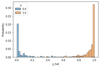
728x90
'딥러닝_Pytorch' 카테고리의 다른 글
| [딥러닝] Pytorch Regression with DNN(Deep Neural Network) (0) | 2022.06.30 |
|---|---|
| [딥러닝-예제] 선형회귀 (Linear Regression+deep neural network) (보스턴 주택가격예측) (0) | 2022.06.29 |
| [딥러닝-예제] 선형회귀 (Linear Regression) (당뇨병 예측) (0) | 2022.06.27 |
| [딥러닝] Mean Square Error (MSE) Loss (0) | 2022.06.27 |
| [딥러닝-예제] 선형회귀 (Linear Regression) (보스턴 주택가격예측) (0) | 2022.06.27 |
'딥러닝_Pytorch' Related Articles
more


Comments